
The table reports whether Medium Scale Travelling Ionospheric Disturbances have been recently detected. Every 15 minutes the status is updated and a new row of the table is displayed, the column entries of the table are here explained: Time (UT) corresponds to the beginning time in UT of the last 45 minutes interval that was evaluated for detecting TIDs (this time also corresponds to the central time of the displayed Doppler shift spectrogram); State reports whether a TID is detected and analyzed. State can assume different values and can be highlighted in different colors according to the potential effect on GNSS users. The possible states are the following:
Horizontal velocity is an apparent horizontal velocity of the analyzed TIDs with respect to the ground.
Azimuth is the azimuth of the TID propagation (0 degrees --> TIDs propagate towards north, 90 degrees --> TIDs propagate towards east, etc. ).
Period is the period of the dominant waves in the last 90-min interval.
Oscillation velocity $ v_{osc} $ (m/s) corresponds to the amplitude of TIDs and is derived estimated from the values of the observed Doppler shifts $ f_{D} $ as $ v_{osc} = { c \cdot f_{D} \over 2f } $, where $c$ is the speed of light and $f$ is the sounding frequency (4.65 MHz). The displayed value is the average RMS value calculated over 90-min interval and three sounding paths. Only TIDs with $ v_{osc} $ > 1.93 m/s (0.06 Hz) are displayed (analyzed). Values exceeding 16 m/s (~0.5 Hz) correspond to significant TIDs.
All these quantities represent average values calculated over the 90-min interval with central time given in the first column. As there is a 15 min time step - overlap of subsequent time intervals over which the quantities are evaluated, the subsequent values might be similar. It is always recommended to look at the Doppler shift spectrogram to see whether approximations of Doppler shift spectrogram by time series of Doppler shifts are meaningful. If TIDs are not analyzed, the N/A values are displayed.
The Doppler shift spectrogram shows an interval of 90 minutes of the latest data.
The recorded data are processed in several steps. The whole calculation is repeated each 15-min, which corresponds to the length of recorded data files.
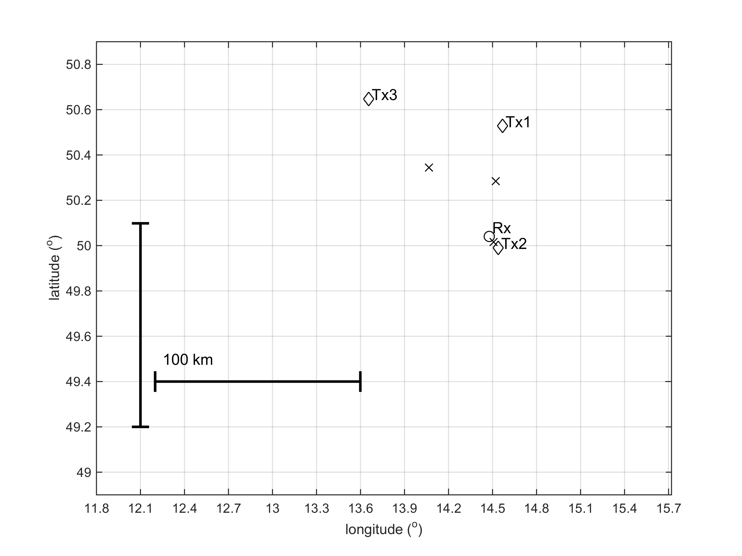
First, Doppler shift spectrograms are computed for the last 90-min record (example in Figure 2). The frequency corresponding to the ground wave is removed from the spectrogram. Then maxima of spectral intensities are searched in three preselected frequency bands that correspond to the frequency bands of the individual transmitter-receiver pairs. The frequencies $ f_{Di} $ corresponding to the maxima of spectral intensities for each transmitter-receiver are stored together with powers $ p_{pi} $ calculated in the narrow frequency band around these maxima (bandwidth on the order of ~0.1 Hz). In addition, powers $ p_{Ti} $ in the whole frequency bands in which the maxima are searched are evaluated (frequency band of about 4 Hz). In addition to the values of $ f_{Di} $ and $ p_{pi} $ the power ratios $ r_{i} = p_{pi} /p_{Ti} $ are also stored to a file with 1-min step (the stored values are 1 min averages). High values of $ r_{i} $ approaching to 1 indicate clear signals suitable for further analysis, whereas low values of $ r_{i} $ indicate signals with insignificant and featureless spectral maxima that occur e.g. during spread F conditions. Such signals are inconvenient for further analysis.
In the next step, the stored values of $ f_{Di} $ , $p_{pi}$ and $r_{i}$ are analyzed. First the offsets are removed and it is worked with values $ f_{DCi} = f_{Di} - < f_{Di} > $ further, where $ < f_{Di} > $ is the mean value over the 90-min intervals.
Next it is decided if TID or spread F likely occurred in the last 45 min and if propagation analysis of the TIDs makes sense in the last 90 min. These decisions are performed by checking if the following criteria are fulfilled.
a) TIDs are likely detected in the last 45 minutes if conditions (1) and (2) are fulfilled
b) Spread F is likely detected in the last 45 minutes if condition (3) is fulfilled at least for 2/3 data points in the last 45 minutes.
$$ ( p_{pi} \gt Th1 ) \quad and \quad ( r_{i} \lt Th2 ) \tag{3} $$
Conditions (3) means that there is relatively large power distributed in relatively large spectral bandwidths.
c) TIDs are only analyzed if condition (1) is fulfilled over the last 90 min; it is required that 7/9 of data points in the last 90 min fulfill the condition (1).
This web page forms part of the European Space Agency's network of space weather services and service development activities, and is supported under ESA contract number 4000134036/21/D/MRP. For further product related information or enquiries contact the helpdesk. E-mail: helpdesk.swe@ssa.esa.int All publications and presentations using data obtained from this site should acknowledge [provider] and The ESA Space Safety Programme For further information about space weather in the ESA Space Safety Programme see: www.esa.int/spaceweather
Access the ESA SWE Portal here: http://swe.ssa.esa.int